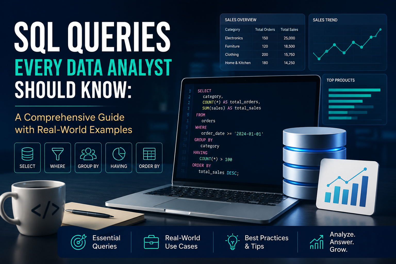
SQL Queries Every Data Analyst Should Know: A Comprehensive Guide with Real-World Examples

As a data analyst, SQL is your most essential tool. While it’s possible to get by with basic `SELECT` statements, truly effective analysis requires a deeper toolkit.

Mastering a core set of SQL queries is what separates analysts who can just retrieve data from those who can uncover actionable insights. This guide covers the essential SQL queries every data analyst should know, from foundational techniques to advanced analytical functions, complete with practical examples you can apply immediately.

1. Getting Started: Data Sampling and Exploration

Before diving into complex analysis, you need to understand your data. These queries help you establish a baseline understanding of your datasets.

Previewing Data with `SELECT` and `LIMIT`

The most common starting point is simply looking at your data. Instead of loading an entire table (which can be slow for large datasets), use `LIMIT` to view a sample .

 `“sql

SELECT *

FROM orders

LIMIT 10;

“`

This query retrieves all columns from the `orders` table but only shows the first 10 rows. It’s perfect for getting a quick sense of column names, data types, and the general structure of your table .

Knowing the Size of Your Table with `COUNT(*)`

Understanding how much data you’re working with is crucial for planning your analysis.

“`sql

SELECT COUNT(*) AS total_orders

FROM orders;

“`

This returns the total number of rows in the table . This simple statistic gives you context for other queries, like knowing whether a subset you’re analyzing represents a meaningful portion of your data.

Finding Unique Values with `DISTINCT`

Categorical columns often contain repeating values. The `DISTINCT` keyword helps you identify what those unique categories are.

“`sql

SELECT DISTINCT payment_method

FROM orders;

“`

For instance, this query will return a list of all the unique payment methods used in your orders table, such as “credit_card”, “paypal”, and “bank_transfer” . This is invaluable for data cleaning, understanding your business dimensions, and preparing for grouping operations .

2. Core Analysis: Filtering, Sorting, and Aggregating

Once you’re familiar with your data, you can begin extracting specific information and summarizing it.

Filtering Data with `WHERE`

Raw data is rarely useful in its entirety. The `WHERE` clause lets you filter rows based on specific conditions .

“`sql

SELECT *

FROM orders

WHERE order_status = ‘Completed’

  AND order_date >= ‘2023-01-01’;

“`

This query retrieves only completed orders from 2023 onward . You can combine conditions with `AND`, `OR`, and use comparison operators like `>`, `<`, and `=` to create precise filters .

Sorting Data with `ORDER BY`

When presenting data or identifying top performers, sorting is essential. The `ORDER BY` clause sorts results in ascending (`ASC`) or descending (`DESC`) order .

“`sql

SELECT customer_id, total_amount

FROM orders

ORDER BY total_amount DESC

LIMIT 5;

“`

This query finds your top 5 highest-spending customers by sorting the total amount in descending order and limiting the result .

Aggregating Data with `GROUP BY` and Aggregate Functions

Aggregation is the heart of analytical reporting. It allows you to summarize data across different groups using functions like `COUNT()`, `SUM()`, `AVG()`, `MIN()`, and `MAX()` .

 “`sql

SELECT

    product_id,

    COUNT(*) AS total_orders,

    SUM(quantity) AS total_units_sold,

    AVG(quantity) AS average_quantity_per_order

FROM order_items

GROUP BY product_id

ORDER BY total_units_sold DESC;

“`

This query groups data by `product_id` and calculates the number of orders, total units sold, and average quantity per order for each product. This is ideal for identifying best-selling products .

Filtering Groups with `HAVING`

The `WHERE` clause filters individual rows before aggregation. The `HAVING` clause, however, filters groups *after* aggregation .

“`sql

SELECT

    product_id,

    SUM(quantity) AS total_units_sold

FROM order_items

GROUP BY product_id

HAVING SUM(quantity) > 100;

“`

This query shows only the products that have sold more than 100 units in total. It’s useful for focusing on high-volume products .

 3. Connecting Data: Joins and Conditional Logic

Real-world data is spread across multiple tables. Connecting them and applying logic is key to powerful analysis.

Combining Tables with `JOIN`

Most business questions require data from more than one table. `JOIN` statements combine rows from two or more tables based on a related column .

“`sql

SELECT

    c.customer_name,

    o.order_id,

    o.total_amount

FROM customers c

JOIN orders o ON c.customer_id = o.customer_id;

“`

This query joins the `customers` and `orders` tables on the `customer_id` column. The result shows customer names alongside their order details, providing a complete picture that neither table can offer alone .

Handling Missing Data with `COALESCE`

Missing or `NULL` data can cause problems in analysis. `COALESCE` returns the first non-NULL value from a list, making it perfect for handling missing values .

“`sql

SELECT

    customer_id,

    COALESCE(phone_number, ‘Not Provided’) AS phone

FROM customers;

“`

 This query replaces any `NULL` phone numbers with the text ‘Not Provided’ .

 Creating New Columns with `CASE`

The `CASE` statement enables conditional logic in your queries, allowing you to categorize data or create new dimensions for analysis .

“`sql

SELECT

    customer_id,

    total_amount,

    CASE

        WHEN total_amount >= 1000 THEN ‘High Value’

        WHEN total_amount >= 500 THEN ‘Medium Value’

        ELSE ‘Low Value’

    END AS customer_segment

FROM orders;

“`

This query creates a new column called `customer_segment` that classifies customers into tiers based on their order total. This is a direct and powerful way to segment your data for deeper analysis .

4. Advanced Analytics: Window Functions and CTEs

When you need to perform sophisticated calculations without collapsing your data, these tools are invaluable.

Performing Calculations with Window Functions

Window functions perform calculations across a set of rows related to the current row. Unlike `GROUP BY`, they do not collapse rows, allowing you to retain individual row details while adding analytical context .

Ranking with `RANK()`:

“`sql

SELECT

    customer_id,

    total_amount,

    RANK() OVER (ORDER BY total_amount DESC) AS rank_position

FROM orders;

“`

This query assigns a rank to each customer based on their `total_amount`. This helps identify your top customers without losing any other order details .

Calculating Running Totals:

“`sql

WITH monthly_report AS (

    SELECT

        DATE_TRUNC(‘month’, order_date) AS month,

        SUM(total_amount) AS monthly_sales_total

    FROM orders

    GROUP BY month

)

SELECT

    month,

    monthly_sales_total,

    SUM(monthly_sales_total) OVER (ORDER BY month) AS running_sales_total

FROM monthly_report

ORDER BY month;

“`

This common table expression (CTE) first calculates monthly sales totals and then applies a window function to create a running total, showing cumulative sales over time .

Structuring Queries with CTEs

Common Table Expressions (CTEs) are temporary result sets that you can reference within a larger query. They make complex queries more readable and easier to debug .

“`sql

WITH high_value_orders AS (

    SELECT *

    FROM orders

    WHERE total_amount > 1000

)

SELECT

    customer_id,

    COUNT(*) AS high_value_order_count

FROM high_value_orders

GROUP BY customer_id

ORDER BY high_value_order_count DESC;

“`

This approach breaks down the problem: the CTE `high_value_orders` first isolates the data we care about, and the main query then performs the analysis on that subset . This modularity is essential for building reliable and scalable analytical queries .

 Conclusion

Mastering these SQL queries will equip you to handle the majority of real-world data analysis tasks. From foundational exploration with `SELECT` and `WHERE` to sophisticated calculations with window functions and CTEs, these tools form the backbone of analytical work .

The best way to solidify these skills is through consistent practice with real datasets. Applying these queries to your own data will transform how you approach analysis and unlock valuable insights to drive decision-making .